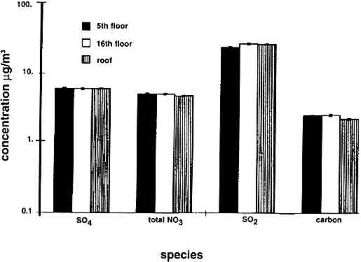
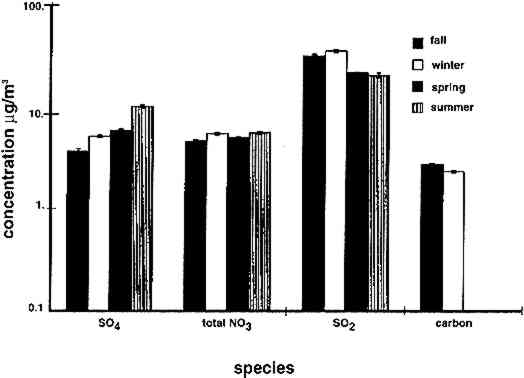
4 RESULTS

4.1 AIRBORNE CONCENTRATIONS OF CHEMICAL SPECIES

Airborne concentrations of SO42− particles, elemental carbon particles, SO2 gas, and total NO3− are shown in figures 5 and 6. Results of SEM analyses of the polycarbonate membrane filters are presented in a separate paper (Etyemezian et al. 1998b). Averages and standard deviations of concentrations are based on the two side-by-side replicate samplers. When one of the replicate samplers malfunctioned, the concentration was obtained from a single sample. The standard deviation for a single sample is approximated by the concentration multiplied by the average coefficient of variation (COV) for all samples for which replicates are available (44 of 48 samples). The COV has been calculated as the standard deviation divided by the average concentration. Each sample has been blank-corrected by subtracting the average mass of analyte found on field blanks from the mass of analyte found on the sample (table 2).

Fig. 5. Concentrations averaged over all four seasons

Fig. 6. Seasonal concentrations averaged over the three sampling locations

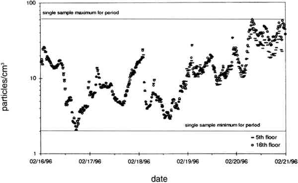
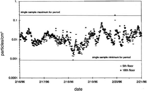
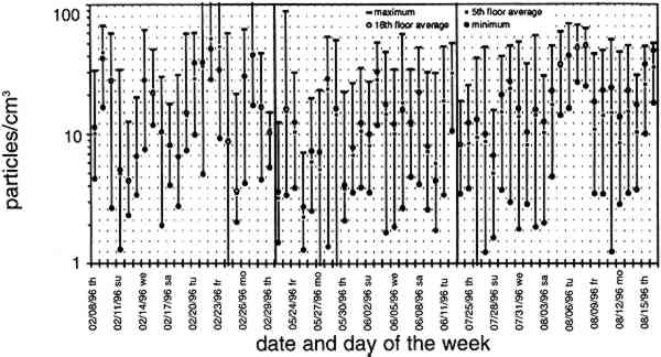
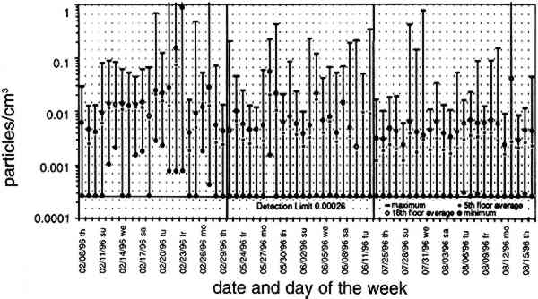
TABLE 2. ANALYTICAL DETECTION LIMITS, AVERAGE SAMPLE MASS, AND AVERAGE FIELD BLANK MASS

Several authors have documented artifacts associated with NO3 species measurement using staged filterpack systems (Appel et al. 1981; Mulawa and Cadle 1985; Hering et al. 1988). For example, volatile NO3− aerosol deposited on Teflon filters may subsequently evaporate. The vapor then redeposits on the downstream nylon filters, resulting in overestimated HNO3 gas and underestimated NO3− particle concentrations. In order to account for possible sampling artifacts, NO3 species concentrations from the experiments reported here are conservatively expressed as total NO3− (HNO3 gas and NO3− particles) by summing values from the Teflon and nylon filters.

SO2 concentrations are based on the chemical analyses of both the nylon and cellulose filters, since the nylon filters tend to remove some SO2 from the airstream (Chan et al. 1986; Cadle and Mulawa 1987). Experiments in the fall of 1995 showed that two sets of cellulose filters may be needed to capture all of the SO2 at high concentrations. Therefore, a second pair of cellulose filters was added downstream of the first set for the latter part of the fall experiments and all remaining runs.

As with the other airborne concentration data presented here, the standard deviations of elemental carbon concentrations reflect the variability between two side-by-side replicate airborne concentration samplers. However, only 10 of the 48 samples and 5 of the 19 field blanks have had replicate chemical analyses. Therefore, the standard deviations of carbon mass on each filter are approximated by the average COV of the samples for which replicate chemical analyses have been performed.

4.2 LASER PARTICLE COUNTS

Examples of particle counts for the period February 16–20, 1996, appear in figure 7. Although particle concentration data are available on a 2-minute average basis, the concentrations in figure 7 have been averaged over 10 minutes to improve legibility. Daily average, maximum, and minimum particle concentrations are plotted in figure 8, and weekday vs. weekend particle concentrations are presented in table 3.

Fig. 7a. Laser particle counts for > 0.5 μm particles, February 16–20, 1996. Major and minor tick marks correspond to midnight and noon of indicated date, respectively. Data have been averaged over 10 minutes for legibility.

Fig. 7b. Laser particle counts for >5 μm particles, February 16–20, 1996. Major and minor tick marks correspond to midnight and noon of indicated date, respectively. Data have been averaged over 10 minutes for legibility.

Fig. 8a. Daily average, maximum, and minimum laser particle counts for > 0.5 μm particles. Maxima on February 21, 22, 23, 27, 1996, are 107, 133, 146, 109 particles/cm3, respectively. Minima on February 24, May 27, 29, and July 26, 1996, are 0.90, 0.66, 0.97, and 0.86 particles/cm3, respectively. Vertical bars extend from minimum to maximum measured concentrations.

Fig. 8b. Daily average, maximum, and minimum laser particle counts for > 5 μm particles. Maxima on February 21, 22, 23, 27, and August 13, 1996, are 1.38, 10.01, 20.35, 1.33, and 3.78 particles/cm3, respectively. Vertical bars extend from minimum to maximum measured concentrations.

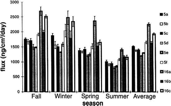
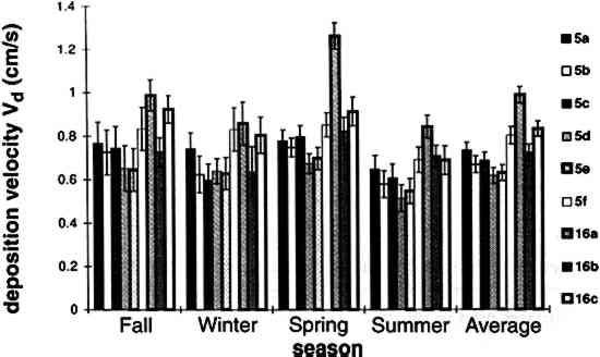
TABLE 3. WEEKDAY, SATURDAY, AND SUNDAY AVERAGE PARTICLE CONCENTRATIONS

4.3 VERTICAL DEPOSITION FLUX AND VERTICAL DEPOSITION VELOCITY

Measured vertical deposition fluxes and deposition velocities appear in figures 9 and 10. SO2 flux averages and standard deviations are based on the four replicate cellulose filters on each Teflon-coated aluminum plate. Vertical deposition flux is a measure of how much SO2 has deposited onto the surrogate surface per unit area per unit time. The deposition velocity Vd is calculated by dividing the deposition flux by the airborne concentration. The average deposition velocity and standard deviation have been calculated using:

Fig. .

Fig. 9. SO2 deposition fluxes

Fig. 10. SO2 deposition velocities

The average airborne concentration C used for calculating Vd on either the 5th or 16th floor is based on the two 1-week airborne concentrations measured on the corresponding floor. It is assumed that this average airborne concentration applies to all of the flux measurement sites on that patio. This is a reasonable assumption based on the agreement between the two replicate sets of filters sampled on each patio.

The surrogate surfaces used in this study are considered to be perfect sinks for SO2, and thus SO2 is assumed to be instantaneously and completely removed when it reaches the filter. The deposition velocity is thus only a measure of gas phase mass transport from the atmosphere to the surrogate surfaces and does not include any possible surface resistance. Since limestone is not a perfect sink for SO2, the deposition velocities to the stone surface will be lower than those measured using surrogate surfaces.