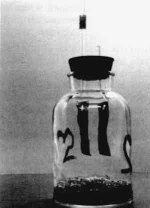
3 EXPERIMENTAL PROCEDURES

CORROSION RATES were measured on clean, smooth coupons of chemically pure “assay” lead foil, cut to a standard size of 73 � 45 mm, with a hole of 8 mm diameter. The lead foil had a thickness of 0.1524 mm (0.006 in). Exposure of the coupons was done in 1000 ml glass bottles, suspended from glass hooks over 50 g (air dry) of the sample material or in empty bottles for the controls. One set of controls was used in every corrosion experiment. The exposure assembly, shown in figure 1, is virtually the same as that used by Clarke and Longhurst (1961) and others (Donovan and Stringer 1971; Donovan and Moynehan 1965). Their results showed that the use of rubber stoppers in the assembly does not accelerate corrosion. In all experiments reported here, except run 6, exposure conditions were 50�C and 80% RH. In experiment 6, temperature was 30�C and the humidity was cycled between 50% and 90% in 12-hour intervals.

Fig. 1. Exposure vessel used for corrosion experiments, with wood product samples and lead coupons in place

The lead coupons were degreased in acetone, pickled in boiling 1% acetic acid to remove all lead salts, rinsed under running water, and dried by dipping in acetone. The cleaning procedure closely follows ASTM standard G1-81 (1981). It was found in preliminary experiments that the suggested cleaning time of 5 minutes was excessive and that a 15-second wash was sufficient to remove all corrosion product, even from moderately corroded coupons. The cleaned coupons were weighed on an analytical balance (Sartorius Selectra) to the nearest 0.0001 g.

The wood product samples were cut into cubes of 1/2 in sides and subsequently comminuted in a Wiley mill to pass a 4 mesh screen. Milling was done to accelerate mixing of the vapors inside the wood with the surrounding air. Samples were weighed into the exposure bottles and kept in a controlled environment cabinet (AMINCO Climate-Lab Assembly) for 5 days before the start of the experiment. It had been shown previously that this time is sufficient for the samples to reach moisture equilibrium (Berndt 1987). At the end of the equilibration period, the bottles were closed with rubber stoppers holding the cleaned and weighed lead coupons and the exposure period started. At the end of the respective exposure times, bottles were withdrawn and the stoppers removed. The lead coupons were allowed to reach temperature equilibrium with the room air and then reweighed. The difference between weight before and after exposure was recorded as the weight gain.

In most experiments, the corroded lead coupons were cleaned again after weighing to determine the weight loss on exposure. As stated in ASTM standard G1-81 (1981), some metal is dissolved in this cleaning process and a correction has to be applied. The coupons were therefore subjected to the cleaning process seven times, and the mass loss plotted against the number of cleaning steps. A sample plot is shown in figure 2. If corrosion product removal is reasonably slow, the plot should show weight loss on washing at two different linear rates: first, a fast weight loss due to salt removal, giving a line through the origin: and second, a slower rate due to metal dissolution. The true weight of corrosion product removed would be the y-value of the intersection of the two lines.

Fig. 2. Example of a plot used for weight-loss determination

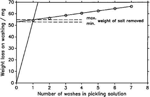
In this study, the line representing metal dissolution was determined by a linear regression on the last five data points of the cleaning series, since visual examination of the plots showed that these lay in all cases on a straight line. In figure 2, all seven points lie nearly on the regression line. This is representative for virtually all determinations carried out. Only when cleaning the most severely corroded coupons was there a significant deviation of the first one or two points from the fitted line. It was impossible in all cases to establish a rate of salt dissolution. As a compromise, a minimum and a maximum weight of the removed corrosion product were determined. The minimum was found from the y-intercept of the line fitted to the last five data points, assuming an infinitely fast rate of salt dissolution. The maximum was taken as the y-value of the intersection of the fitted line with the line through the origin and the first data point (fig. 2). Weight loss on exposure was calculated by subtracting the weight of salt removed from the weight after exposure and subtracting the result from the initial weight of the lead coupon.

As mentioned above, in all cases all points of the weight loss determination plots lay nearly on the metal-dissolution line. It can be assumed that the minimum weight loss is much closer to the true value than the maximum. Also, minimum and maximum weight loss rarely differed by more than the experimental error. Calculations and analyses were therefore based on minimum weight loss data.

The pH-values of the wood products, listed in table 1, were determined following the procedure outlined by Miles (1986). Twenty-five cc of the Wiley-milled samples and 150 cc of distilled water were agitated with a magnetic stirrer for 2 hours. After this time, the pH was measured with a Beckman pHI 45 pH meter by immersing a Beckman Futura II combination glass electrode and a thermocompensator in the stirred suspension and noting the stable instrument reading. Standard Beckman buffers of pH 4 (phthalate) and 7 (phosphate) were used for calibration. The reported values are averages of two independent measurements. Duplicate determinations did not vary by more than 0.05 pH units.

TABLE 1 Explanation of Sample Codes