Solubility Parameters: Theory and Application
John BurkeThe division of the Hildebrand parameter into three component Hansen parameters (dispersion force, polar force, and hydrogen bonding force) considerably increases the accuracy with which non-ionic molecular interactions can be predicted and described. Hansen parameters can be used to interpret not only solubility behavior, but also the mechanical properties of polymers, pigment binder relationships, and the activity of surfactants and emulsifiers.
Being a three component system, however, places limitations on the ease with which this information can be practically applied. Translating this three component data onto a two-dimensional graph (by ignoring one of the components) solves this problem but sacrifices a certain amount of accuracy at the same time. What is needed is a simple, planar graph on which polymer solubility areas can be drawn in their entirety in two dimensions. A triangular graph meeting these qualifications was introduced by Jean P. Teas in 1968, using a set of fractional parameters mathematically derived from the three Hansen parameters. Because of its clarity and ease of use, the Teas graph has found increasing application among conservators for problem solving, documentation, and analysis, and is an excellent vehicle for teaching practical solubility theory.
In order to plot all three parameters on a single planar graph, a certain departure must be made from established solubility theory. The construction of the Teas graph is based on the hypothetical assumption that all materials have the same Hildebrand value. According to this assumption, solubility behavior is determined, not by differences in total Hildebrand value, but by the relative amounts of the three component forces (dispersion force, polar force, and hydrogen bonding force)that contribute to the total Hildebrand value. This allows us to speak in terms of percentages rather than unrelated sums.
Hansen parameters are additive components of the total Hildebrand value (Equation 6). In other words, if all three Hansen values (squared) are added together, the sum will be equal to the Hildebrand value for that liquid (squared). Teas parameters, called fractional parameters, are mathematically derived from Hansen values and indicate the percent contribution that each Hansen parameter contributes to the whole Hildebrand value:
![]()
![]()
For example, the alkanes, with intermolecular attractions due entirely to dispersion forces, are represented by a dispersion parameter of 100, indicating totality, with both polar and hydrogen bonding parameters of zero. Molecules that are more polar have dispersion parameters of less than 100, the remainder proportionately divided between polar and hydrogen bonding contributions as the particular Hansen parameters dictate.
Because Hildebrand values are not the same for all liquids, it should be remembered that the Teas graph is an empirical system with little theoretical justification. Solvent positions were originally located on the graph according to Hansen values (using Equation 8), and subsequently adjusted to correspond to exhaustive empirical testing. This lack of theoretical foundation, however, does not prevent the Teas graph from being an accurate and useful tool, perhaps the most convenient method by which solubility information can be illustrated. Fractional parameters for solvents are listed in Table 6, at the end of this paper.
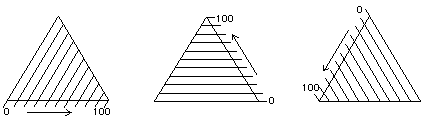
Figure 8.
The Teas graph is an overlay of three solubility scales.
The layout of a triangular graph is confusing at first to people who are accustomed to the common cartesian rectangular coördinate graph. Instead of two axes perpendicular to each other, there are three axes oriented at 60°, and instead of these three axes requiring three dimensions in space, the triangular graph is flat. Furthermore, on a cartesian graph all the scales graduate out from the same origin, but on a triangular graph the zero point of any one scale is the upper limit of another one.
This unusual construction derives from the overlay of three identical scales, each proceeding in a different direction (Figure 8). In this way, any point within the triangular graph uses three coördinates, the sum of which will always be the same: 100 (Figure 9).
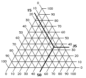
Figure 9 At any point on a triangular graph, all three
coördinates add up to 100.
By means of a triangular graph, solvents may be positioned relative to each other in three directions (Figure 10).
Sorry, as of 2/5/96, Figure 10 is not yet available
Alkanes, whose only intermolecular bonding is due to dispersion forces, are located in the far lower right corner of the Teas graph, the corner that corresponds to 100% dispersion force contribution, and 0% contribution from polar or hydrogen bonding forces. Moving toward the lower left corner, corresponding to 100% hydrogen bonding contribution, the solvents exhibit increasing hydrogen bonding capability, culminating at the alcohols and water, molecules with relatively little dispersion force compared to their very great hydrogen bonding contribution. Moving from the bottom of the graph upwards we encounter solvents of increasing polarity, due less to hydrogen bonding functional groups than to an increasingly greater dipole moment of the molecule as a whole, such as the ketones and nitro compounds.
Overall, the solvents are grouped closer to the lower right apex than the others. This is because the dispersion force is present in all molecules, polar or not, and determining the dispersion component is the first calculation in assigning Hansen parameters, from which the Teas fractional parameters are derived. Unfortunately, this greatly overemphasizes the dispersion force relative to polar forces, especially hydrogen bonding interactions.
Figure 11 illustrates solvents on a Teas graph grouped according to classes. Increasing molecular weight within each class shifts the relative position of a solvent on the graph closer to the bottom right apex. This is because, as molecular weight increases, the polar part of the molecule that causes the specific character identifying it with its class, called the functional group, is increasingly "diluted" by progressively larger, nonpolar "aliphatic" molecular segments. This gives the molecule as a whole relatively more dispersion force and less of the polar character specific to its class.
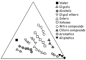
Figure 11 Solvents grouped according to classes. Within each class,
increasing molecular weight shifts the solvent position toward the
right axis, corresponding to an increase in dispersion contribution
relative to polar contributions.
This trend toward less polarity with increasing molecular weight within a class also accounts for the observation that lower molecular weight solvents are often "stronger" than higher molecular weight solvents of the same class, although determinations of solvent strength must really be made in terms of the solvents position relative to the solubility area of the solute. (Another reason for low molecular weight solvents seeming more active is that smaller molecules can disperse throughout solid materials more rapidly than their bulkier relatives.)
The only class in which increasing molecular weight places the solvent further away from the lower right corner is the alkanes. As previously stated, the intermolecular attractions between alkanes are due entirely to dispersion forces, and accordingly, Hansen parameter values for alkanes show zero polar contribution and zero hydrogen bonding contribution. Since fractional parameters are derived from Hansen parameters, one would expect all the alkanes to be placed together at the extreme right apex.
Observed behavior indicates, however, that different alkanes do have different solubility characteristics, perhaps because of the tendency of larger dispersion forces to mimic slightly polar interactions. For this reason, Teas adjusted the locations of the alkanes to correspond to empirical evidence, using Kauri-Butanol values to assign alkane locations on the graph. Several other solvent locations were also shifted slightly to properly reflect observed solubility characteristics. The position of water on the chart is very uncertain, due to the ionic character of the water molecule, and the placement in this paper is according to recent published values (Teas, 1976). The presence of water in a solvent blend, however, can alter dramatically the accuracy of solubility predictions.
[It should be noted that the position of methylene chloride is also correct according to recent values. Many earlier publications have given methylene chloride incorrect parameters properly corresponding to Hansen's values for methyl chloride, a different chemical, possibly due to calculation error.]
Given the solvent positions, it is possible to indicate polymer solubilities using methods similar to those used by Crowley and Hansen: a polymer is tested in various solvents, and the results indicated on the graph (a 3-D model is no longer necessary). At first, individual liquids from diverse locations on the graph are mixed with the polymer under investigation, and the degree of swelling or dissolution noted. Liquids that are active solvents, for example, might have their positions on the graph marked with a red dot. Marginal solvents might be marked with a yellow dot, and nonsolvents marked with black. Once this is done, a solid area on the Teas graph will contain all the red dots, surrounded with yellow dots (see Figure 12).
The edges of this area, or polymer solubility window, can be more closely determined in the following way. Two liquids near the edge of the solubility window are chosen, one within the window (red dot), and one outside the window (black dot). Dissolution (or swelling) of the polymer is then tested in various mixtures of these two liquids, using cloud-point determinations if accuracy is essential, and the mixture just producing solubility is noted on the graph, thus determining the edge of the solubility window. (The mixture would be located on a line between the two liquids, at a point corresponding in distance to the ratio of the liquids in the mixture.) If this procedure is repeated in several locations around the edge of the solubility window, the boundaries can be accurately determined. Interestingly, some composite materials (such as rubber/resin pressure sensitive adhesives, or wax resin mixtures) can exhibit two or more separate solubility windows, more or less overlapping, that reflect the degree of compatibility and the concentration of the original components.
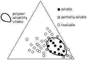
Figure 10 The solubility window of a hypothetical polymer
(circles indicate solvents).
This method of solubility window determination can be performed on samples under a microscope, and the results plotted on a Teas graph. In cases where the solubilities of artifactual materials are to be assessed prior to treatment, it is often unnecessary to delineate the entire solubility window of the materials in question. It can suffice to record the reaction of the materials to the progressive mixtures of a few selected solvents under working conditions in order to determine appropriate working solutions.
The solubility window of a polymer has a specific size, shape, and placement on the Teas graph depending on the polarity and molecular weight of the polymer, and the temperature and concentration at which the measurements are made. Most published solubility data are derived from 10% concentrations at room temperature.
Heat has the effect of increasing the size of the solubility window, due to an increase in the disorder (entropy) of the system. The more disordered a system is (increased entropy), the less it matters how dissimilar the solubility parameters of the components are. Since entropy also relates to the number of elements in a system (more elements=more disorder), polymer grades of lower molecular weight (many small molecules) will have larger solubility windows than polymer grades of higher molecular weight (fewer large molecules).
Concentration also has an effect on solubility. As stated, most polymer solubility windows are determined at 10% concentration of polymer in solvent. Because an increase in polymer concentration causes an increase in the entropy of the system (more elements=more disorder), solubility information can be considered accurate for solutions of higher concentration as well. Solvent evaporation as a polymer film dries serves to increase the polymer concentration in the solvent, thus insuring that the two materials stay mixed. It is possible, however, for polymer solutions of less than 10% to phase separate (become immiscible), due to a decrease in entropy. This is particularly likely with polymer-solvent combinations at the edge of the polymer solubility window. In other words, with lower polymer concentration there is an increase in the order of the system (less entropy); therefore, the size of the solubility window becomes smaller (there is less difference tolerated between solvent and polymer solubility values).
Solution viscosity also varies depending on where in the polymer solubility window the solvent is located. One might expect viscosity to be at a minimum when a solvent near the center of a polymer solubility window is used. However, this is not the case. Solvents at the center of a polymer solubility window dissolve the polymer so effectively that the individual polymer molecules are free to uncoil and stretch out. In this condition molecular surface area is increased, with a corresponding increase in intermolecular attractions. The molecules thus tend to attract and tangle on each other, resulting in solutions of slightly higher than normal viscosity.
When dissolved in solvents slightly off-center in the solubility window, polymer molecules stay coiled and grouped together into microscopic clumps which tend to slide over one another, resulting in solutions of lower viscosity. As solvents nearer and nearer the edge of the solubility window are used to dissolve the polymer, however, these clumps become progressively larger and more connected and viscosity again increases until ultimately polymer-liquid phase separation occurs as the region of the solubility window boundary is crossed.
The position of a solvent in the solubility window of a polymer has a marked effect on the properties of not only the polymer-solvent solution, but on the dried film characteristics of the polymer as well. Because of the uncoiling of the polymer molecule, films (whether adhesives or coatings) cast from solvent solutions near the center of the solubility window exhibit greater adhesion to compatible substrates. This is due to the increase in polymer surface area that comes in contact with the substrate. (Hildebrand parameters can be related to surface tension, and adhesion is greatest when the polarities of adhesive and adherend are similar.)
Many other properties of dried films, such as plastic crazing or gas permeability are related to the relative position that the original solvent occupied in the solubility window of the polymer. The degree of both crazing and permeability is predictably less when solvents more central to the solubility window have been used.
Solvent evaporation rates can also have a marked affect on dried film properties. The solubility parameters of solvent blends can change during film drying because of the difference in evaporation rates of the component liquids. If a volatile true solvent is mixed with a slow evaporating non-solvent, the compatibility between solvents and polymer can shift as the true solvent evaporates. The predominance of the non-solvent during the last stages of drying can result in a discontinuous, porous film with higher opacity and decreased resistance to water and oxygen deterioration. (There may be instances where these properties are desirable.)
This can be avoided, however, by either blending a small amount of a high boiling true solvent into the solvent mixture (this solvent remains to the last and insures miscibility), or by making sure that, if an azeotropic mixture is formed on evaporation, the parameters of the azeotrope lie within the polymer solubility window.
An azeotrope is a mixture of two or more liquids that has a constant boiling point at a specific concentration. When two liquids are mixed that are capable of forming an azeotrope, the more volatile liquid will evaporate more quickly until the concentration reaches azeotropic proportions. At that point, the concentration will remain constant as evaporation continues. If the position of the azeotropic mixture lies within the solubility window, compatibility with the polymer will continue throughout the drying process. This can be determined by consulting a table of azeotropes and checking the location of the mixture on the Teas graph in relation to the polymer solubility window. (Methods of plotting solvent mixtures are described in the next section.)
Teas graph is particularly useful as an aid to creating solvent mixtures for specific applications. Solvents can easily be blended to exhibit selective solubility behavior (dissolving one material but not another), or to control such properties as evaporation rate, solution viscosity, degree of toxicity or environmental effects. The use of the Teas graph can reduce trial and error experimentation to a minimum, by allowing the solubility behavior of a solvent mixture to be predicted in advance.
Because solubility properties are the net result of intermolecular attractions, a mixture with the same solubility parameters as a single liquid will, in many cases, exhibit the same solubility behavior. Determining the solubility behavior of a solvent mixture, therefore, is simply a matter of locating the solubility parameters of the mixture on the Teas graph. There are two ways by which this may be accomplished: mathematically, by calculating the fractional parameters of the mixture from the fractional parameters of the individual solvents, and geometrically, by simply drawing a line between the solvents and measuring the ratio of the mixture on the graph. The mathematical method is the most accurate, and is appropriate for mixtures of three or more solvents. The geometrical method is the most convenient and is suitable for mixtures of two solvents, or for very rough guesses when three solvents are involved.
The solubility parameter of a mixture of liquids is determined by calculating the volume-wise contributions of the solubility parameters of the individual components of the mixture. In other words, the fractional parameters for each liquid are multiplied by the fraction that the liquid occupies in the blend, and the results for each parameter added together. For example, given a mixture of 20% acetone and 80% toluene:
| fd | fp | fh | |
|---|---|---|---|
| Acetone: | 47 (x .20) = 9.4 | 32 (x .20) = 6.4 | 21 (x .20) = 4.2 |
| Toluene: | 80 (x .80) = 64.0 | 7 (x .80) = 5.6 | 13 (x .80) = 10.4 |
| 20/80 Mix: | fd = 73.4 | fp = 12.0 | fh = 14.6 |
In this way, the position of the solvent mixture can be located on the Teas graph according to its fractional parameters. Calculations for mixtures of three or more solvents are made in the same way.
The geometric method of locating a solvent mixture on the Teas graph involves simply drawing a line between the two solvents in the mix, and finding the point on the line that corresponds to the volume fractions of the mixture.
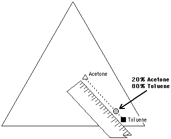
Figure 13 A mixture of 20% acetone and 80% toluene can be located on
the Teas graph by using a pencil and ruler. The mixture lies on a
line connecting the two liquids, at a distance equal to the ratio of
the mixture, and closer to the liquid present in the greatest
amount.
This is illustrated in Figure 13 for the same 20% acetone, 80% toluene mixture. A line connecting acetone and toluene is drawn on the Teas graph. A point is then located on the line, 20% of the length of the line away from toluene. It is important to remember that the location of a mixture will be closer to the liquid present in the greatest amount.
What is interesting about visualizing solvent blends on the Teas graph is the control with which effective solvent mixtures can be formulated. For example, two liquids that are non-solvents for a specific polymer can sometimes be blended in such a way that the mixture will act as a true solvent. This is possible if the graph position of the mixture lies inside the solubility window of the polymer, and is most effective if the distance of the non-solvents from the edge of the solubility window is not too great. This is illustrated in Figure 14a.
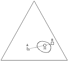
Figure 14a A mixture (M) of non-solvents (A,B) may act as a
true solvent for a polymer if the mixture is located inside the
solubility window for the polymer on the Teas graph.
This phenomenon is particularly valuable when selective solvent action is required. Often it is necessary to selectively dissolve one material while leaving other materials unaltered, as in the case of removing the varnish from a painting, some adhesive tape from the image area of a print, or when a consolidant must not dissolve the material being consolidated. Sometimes the solubilities of all the materials involved are so similar that selecting an appropriate and safe solvent can be difficult. In such cases it is helpful to indicate the solubility windows of both the material that needs to be dissolved (varnish, adhesive, consolidant), and the materials that must be protected (media), on a Teas graph. This can be accomplished by simple solubility testing, noting the results of the tests on the graph.
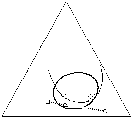
Figure 14b In situations where one material must be dissolved
(dark circle) while another must remain unaffected (shaded area), it
is helpful to plot the solubility of both materials on the graph. A
solvent blend can then be formulated (triangle) that selectively
dissolves only the proper material (see text).
Once this has been done, it is easy to see the overlap of solubilities, and the areas where solubilities are mutually exclusive, if they exist. A solvent blend can then be formulated that actively dissolves the proper material, while positioned as far away from the solubility window of the other material as possible (Figure 14b). It is important to remember that differences in evaporation rates can shift the solubility parameter of the blend as the solvents evaporate, and this must be taken into account. Additionally, while a material may not shown signs of solution in a solvent or solvent blend, the solvent may still adversely affect the material, for example by softening the material or leaching out low molecular weight components. Such changes can be irreversible and must be considered prior to embarking on a treatment.
Although the Teas graph is useful and informative when dealing with complex solubility questions, in most day to day situations choosing a solvent is a straightforward procedure that would be unnecessarily complicated by having to plot entire solubility windows. In most cases, the degree of solubility of a material is simply tested in various concentrations of two or three solvents, in order to determine the mildest solvent capable of forming a solution. Perhaps the most often used solvent mixtures are blends of aliphatic and aromatic hydrocarbons, sometimes with the addition of acetone. This is because the search for the mildest solvent is often synonymous with the search for the least polar solvent (and the aliphatic hydrocarbons are the least polar possible).
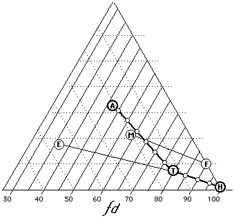
Figure 15
Some common solvent blends (A=acetone, T=toluene, H=heptane,
E=ethanol, M=methylene chloride, F=Freon TF). In most cases,
dispersion force values give a relative indication of solvent
strength (100=weakest, 30=strongest).
Testing whether a polymer is suitable for use in conservation, for example, usually involves determining the mildest solvent mixture that will dissolve both aged and un-aged samples. For this purpose, various concentrations of toluene in cyclohexane are used; should the polymer prove insoluble in straight toluene, however, increasing amounts of acetone are added until solubility is achieved. This type of solubility test anticipates the choices that will be made in working situations.
Looked at in terms of fractional parameters, what is being determined in such tests is essentially the location of the edge of the solubility window for the polymer in relation to the lower right corner of the Teas graph. Figure 15 illustrates various mixtures of heptane, toluene, and acetone. It can been clearly seen that solvent strength increases with greater distance from the 100% dispersion axis. Blends of trichlorotrifluoroethane (FreonTF) and methylene chloride as well as blends of toluene ethanol are also illustrated. In all cases, increasing solvent strength follows decreasing dispersion force contribution.
For this reason, the use of fractional dispersion values (Table 5) is an excellent method for concisely designating relative solvent strength, in place of other more limited scales (Kauri-Butanol number, aromatic content, etc.). The benefits of this approach include the use of a standard designation that encompasses the entire range of solvent strengths, and the ability to easily enlarge the designation to include more precise solubility parameter data if necessary.
| % Heptane | % Toluene | % Acetone | Approx. d |
| 100 | 0 | 0 | 100 |
| 75 | 25 | 0 | 95 |
| 50 | 50 | 0 | 90 |
| 25 | 75 | 0 | 85 |
| 0 | 100 | 0 | 80 |
| 0 | 85 | 15 | 75 |
| 0 | 70 | 30 | 70 |
| 0 | 55 | 45 | 65 |
| 0 | 40 | 60 | 60 |
| 0 | 25 | 75 | 55 |
| 0 | 10 | 90 | 50 |
| 0 | 0 | 100 | 47 |
As we have shown, the Teas graph can can be a useful guide in tailoring solvent blends to suit specific applications. By adjusting the position of the blend relative to the solubility window of a polymer such properties as solution viscosity and adhesion can be optimized. Evaporation rates can be controlled independently of solvent strength, and the effects of temperature and concentration can be anticipated.
A further advantage that can be derived from this latitude in creating solvent mixtures is the possibility of choosing solutions based on degree of toxicity. A solvent mixture having a graph position close to another solvent will have such similar solubility characteristics to that solvent that it can be used interchangeably in many applications. For example, a petroleum solvent of 30% aromatic character is more or less the same whether the aromatic content is due to benzene (very toxic) or to toluene (moderately toxic). By extension, a mixture of ethanol/toluene 50:50 might be used in place of tetrahydrofuran in some applications, and toluene might be replaced with a 3:1 mixture of Stoddard solvent and acetone. In such cases, it should be pointed out that the similarity between solvents and blends having the same numerical parameters decreases as the distance between the components of the blend increases. Where alternate blends are effective, however, the use of a less toxic replacement can be a sensible choice, and the Teas graph a useful tool.
The theory of solubility parameters is a constantly developing body of scientific concepts that can be of immense practical assistance to the conservator. Through the media of solubility maps, complex molecular interactions can be visualized and understood, and in this way, solubility theory can simply function as a ladder to be left behind once the basic concepts are assimilated. On the other hand, the solution to an unusual problem can often be put within reach by graphically plotting solubility behavior on a Teas graph.
In the near future, the extension of solubility theory to encompass ionic and water based systems is conceivable, and the development of simple computer programs to manipulate multi-component solubility parameter data, along with accessible data bases of material solubilities, is probable. Until that time, both conservators and the objects in their charge can continue to profit by the use, either conceptual or real, of solubility parameter theory.
John Burke, The Oakland Museum of California, August 1984Next: References