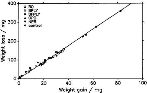
5 RESULTS AND DISCUSSION

IF THE product of atmospheric lead corrosion is the same under all conditions, a plot of weight loss after exposure and cleaning against weight gain after exposure should yield a straight line through the origin. Figure 3 shows that this is indeed the case. Deviations from that line are of the order of magnitude of the experimental error. The slope of the line, the constant weight loss/weight gain ratio, is 4.387. Since the weight loss is equal to the mass of lead cations in the salt formed, and the weight gain is equal to the mass of salt anions, the weight gain/weight loss ratio is characteristic of the salt composition (Berndt 1987). The observed ratio is close to that expected for basic lead carbonate (2PbCO3Pb(OH)2, 4.02). It is significantly higher than for lead formate (Pb(HCOO)2, 2.3) or lead acetate (Pb(CH3COO)2, 1.75). This conforms with observations by Donovan and Moynehan (1965), who found that organic acid anions in salts formed over air drying paints made up about 0.02%–0.20% (by weight) of the salt. These organic acid anions were confined to the layer in intimate contact with the metal (Donovan and Stringer 1971).

Fig. 3. Weight loss of exposed and cleaned lead coupons vs. their weight gain after exposure. See table 1 for explanations of the sample codes.

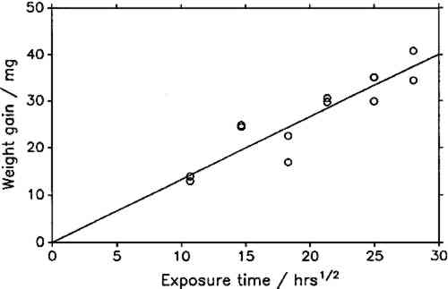
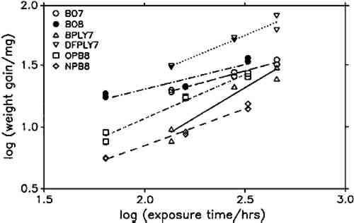
The constant weight loss/weight gain ratio also indicates that the corrosion mechanism was the same in all experiments. The corrosion rate is therefore a valid indicator of the organic acid concentration and atmospheric corrosiveness.

Since the weight gain is more than four times greater than the weight loss, it could be expected that weight gain determinations are more reliable because the weighing error is relatively smaller. That was found not to be the case. Errors from both types of determinations had the same relative magnitude, indicating that the observed errors are not due to lack of weighing precision but are caused by other variables, such as composition and temperature of the test atmosphere or state of the metal surface. Corrosion rates reported here were calculated from weight gain determinations.

Oak wood is known to corrode lead readily and was therefore chosen as the initial test material. It was found that the weight gain of lead on exposure to oak was proportional to the square root of exposure time (fig. 4). It was necessary to find out whether this is true for all other tested materials, that is, whether the value of b in equation 1 is 0.5 in all cases. Taking the logarithms of both sides of equation 1 yields:

Fig. .

Fig. 4. Weight gain of lead coupons exposed over California black oak vs. the square root of the expsure time

Fig. 5. Log-log plot of weight gain vs. exposure time, used to determine the exponent in the power law (weight gain) = (c) (exposure time)b. See table 1 for explanations of the sample codes.

Fig. 6. Comparison of values of the power law exponent b found for different wood products in different corrosion experiments. See table 1 for explanations of the sample codes.

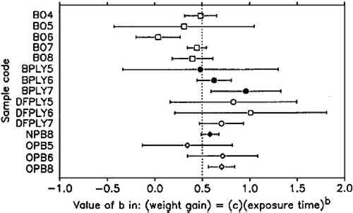
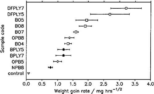
To compare corrosion rates caused by different wood products, the calculated weight gains were plotted against the square root of time and the best slope through the points was determined. The slopes (i.e., the corrosion rate constants) and their 95% confidence intervals for all comparable tests are presented in figure 7. Douglas fir plywood was clearly the most corrosive, and the recently purchased particleboard sample was the least corrosive of all tested wood products. Both results come as a surprise, given the bad reputations of particleboard and oak wood. A comparison of the pH values of the tested wood products (see table 1) with the corresponding corrosion rates confirms (cf. Donovan and Moynehan 1965) that pH is not an indicator of atmospheric corrosiveness.

Fig. 7. Comparison of weight gain rates caused by various wood products in different corrosion experiments, with the assumption of a constant power law exponent, b = 0.5. See table 1 for explanations of the sample codes.

No attempts were made to characterize the samples further than by type of product, pH, and wood species, as given in table 1, since this series of experiments was planned as a trial for the feasibility and sensitivity of this atmospheric corrosion test. The results reported here cannot be generalized with regard to wood species, product, length of storage, or other independent factors.

It appears that corrosive emissions increase with the time between sample preparation (cutting and milling) and the corrosion tests. Birch plywood gave the same corrosion rate in two successive tests, but the other duplicates from identical batches (BO4/BO5, BO7/BO8, DFPLY5/DFPLY7, OPB5/OPB8), all have a higher corrosion rate in the later test. This phenomenon should be investigated systematically in future experiments.

Figure 5 shows that the experimental error of the corrosion rate determination is roughly proportional to the rate itself and usually of acceptable magnitude. In all experiments so far, the test had to be terminated for a given exposure bottle to measure weight changes. This significantly limited the number of experimental points available for corrosion rate determinations, from as low as two test coupons each at two exposure times (all materials in run 5) to at most two test coupons each after six exposure times. As mentioned above, the corrosion rate can be confidently determined and compared for various materials on the basis of weight gain measurements alone. It is therefore possible to make use of continuous weight gain measurement, for example, by suspending the test coupons from an automatic balance. This would increase the number of experimental points available for the rate determination significantly and could be expected to narrow the confidence interval for the calculated rate.

It was originally planned to correlate the corrosion rate in the presence of wood products to that in the laboratory atmosphere at the same temperature and humidity to correct for differences in the “background” corrosiveness (Berndt 1987). This plan proved to be impractical, since the error in the background corrosion rate determinations was greater than any differences found in four experiments. Weight changes were clearly measurable, however, even in the controls.