ABSTRACT—A simple method for testing corrosiveness of atmospheres containing organic acids is presented. Testing is done by exposing lead coupons to the environment of interest at 50�C and 80% RH. Following the weight gain of lead test coupons continuously (e.g., by suspending them from an automatic balance in the test environment) provides a simple and convenient method of evaluating atmospheric corrosiveness. The ratio of cation mass to anion mass in the salt formed due to corrosion over various wood products was the same under all test conditions. The magnitude of this constant ratio suggests that basic lead carbonate (2PbCO3Pb(OH)2) is the principal corrosion product.

1 INTRODUCTION

ENVIRONMENTAL CONDITIONS affect the deterioration rate of artifacts. To know how much, one needs a measure of that rate. Many effects of environmental conditions on artifacts have been discussed qualitatively in the literature (e.g., Thomson 1978). Assessment of the chemical composition of museum environments is a topic of current conservation research (e.g., G.C.I. Newsletter 1988). Interest has focussed on the microclimate created in storage and display containers, partly because it offers good prospects for tight control of conditions, and partly because practical experience showed this to be a significant problem area (Oddy 1973, 1975; Blackshaw and Daniels 1978; Blackshaw 1982; Padfield et al. 1982; G.C.I. Newsletter 1987).

The corrosiveness of microclimates in the vicinity of wood and wood products has long been known and frequently discussed in the literature (Oddy 1973, 1975; Blackshaw and Daniels 1978; Blackshaw 1982; Padfield et al. 1982; FitzHugh and Gettens 1971; Arni et al. 1965a, 1965b; Packman 1960; Clarke and Longhurst 1961; Packman 1957; Donovan and Stringer 1969, 1971). The deleterious agents in these microclimates are organic acids. Acetic acid is the main agent (FitzHugh and Gettens 1971; Arni et al. 1965a, 1965b; Packman 1960; Clarke and Longhurst 1961; Packman 1957; Donovan and Stringer 1969, 1971), but formic, butyric and propionic acid have also been detected (Arni et al. 1965b; Donovan and Stringer 1969, 1971). Formaldehyde also is present over wood-based materials, as well as over many paints and varnishes. Aldehydes are easily oxidized to the corresponding organic acids on metal surfaces by atmospheric oxygen, thereby adding to the overall organic acid concentration. The deleterious effects of formaldehyde have received significant attention in the conservation literature (Carpenter and Hatchfield 1985; Hatchfield and Carpenter 1986; Leveque 1986; Conolly 1987).

Two approaches to quantifying atmospheric corrosiveness are possible: 1) determination of atmospheric composition, and 2) measurement of the corrosion rate caused by the atmosphere of interest. The first approach clarifies the reasons for atmospheric corrosiveness; the second quantifies the rate of the deterioration process. Results obtained by the second approach are directly related to the atmospheric composition, but the forms of the relations have to be determined experimentally. Research into the analysis of microclimate composition is under way elsewhere (G.C.I. Newsletter 1988, 1987). The topic of this article is the determination of atmospheric corrosion rates in microclimates dominated by the presence of wood or wood products, closely following ASTM standards G50–76 and G1-81 (1981).

2 MEASURING THE CORROSIVENESS OF MICROCLIMATES CREATED BY WOOD AND WOOD PRODUCTS

THE PROBLEMS occurring with objects stored in wood-based containers have been reviewed previously (FitzHugh and Gettens 1971; Berndt 1987). Typical degradation processes, for example, formation of efflorescence on calcareous materials (FitzHugh and Gettens 1971) and lead corrosion (Oddy 1973, 1975; Blackshaw and Daniels 1978; Blackshaw 1982; Padfield 1982; FitzHugh and Gettens 1971; Arni et al. 1965a, 1965b; Packman 1960; Clarke and Longhurst 1961; Packman 1957; Donovan and Stringer 1969, 1971; Carpenter and Hatchfield 1985; Hatchfield and Carpenter 1986; Leveque 1986; Berndt 1987; Thomson 1978), are catalyzed by organic acids. For the conservator, catalytic action is especially undesirable because small amounts of the catalyst may have significant degradative effects and because the deleterious agent is not consumed in the degradation process. The latter is useful for an analysis of the environment by deterioration rate measurements because the exposed test material will change the environment only negligibly.

The undesirable action of organic acids in the museum environment stems from the high solubility of most of their metal salts (Weast 1979). While calcium carbonate, the main constituent of sea shells and other calcareous materials, is insoluble in water, calcium acetate is soluble. Dissolution of calcium acetate, relocation, and redeposition on drying caused the calclacite efflorescence seen on several museum objects (FitzHugh and Gettens 1971). Similarly, catalysis of metal corrosion by organic acid vapors proceeds by metal oxide dissolution in the anodic areas of the metal surface. The dissolved organic acid salts migrate to the relatively alkaline cathodic areas, where they hydrolyze and form metal hydroxide (Donovan and Stringer 1971; Scully 1975). The hydroxide may become less soluble by carbonation. In lead corrosion, this leads to the formation of basic lead carbonate, or white lead, as the principal product (Oddy 1973, 1975; FitzHugh and Gettens 1971; Donovan and Stringer 1971; Berndt 1987).

Of the organic acid vapor-induced degradation processes mentioned above, only metal corrosion is readily quantifiable. Calclacite efflorescence on calcareous materials involves a relocation of material only, which depends largely on condensation/evaporation cycles and is not sensitive enough to the amount of organic acids present. Zinc and lead are the metals most susceptible to organic acid vapor corrosion (Donovan and Stringer 1969, 1971). Comparing the solubilities of zinc and lead chlorides to the solubilities of the respective organic acid salts (Weast 1979) suggests that zinc is also very vulnerable to hydrochloric acid vapors while lead is not. The specificity of lead to corrosion by organic acids makes it the metal of choice for an atmospheric corrosiveness indicator.

Metal corrosion rate is measured as the amount of metal converted to metal salt per unit time and per unit area of exposed surface. To be a useful indicator, corrosion rate has to increase monotonically with increasing organic acid concentration. This is likely unless the corrosion mechanism changes at some concentration. A change in corrosion mechanism usually leads to a change in the corrosion product formed (Clarke and Longhurst 1961). If the corrosion product formed is the same in all exposure tests, the corrosion rate is a valid indicator of acid concentration.

Metal corrosion rate is commonly determined by exposing a cleaned test coupon with known surface area and weight to the conditions of interest for a length of time, removing the salt formed by an appropriate method, and determining the weight loss. Dividing the weight loss by the exposed surface area and the exposure time gives the corrosion rate (ASTM 1981). If the salt formed is the same under all conditions and if it does not separate from the test coupon during the test period, the weight gain on exposure can be used for corrosion rate determination. Following weight gain has the advantage of eliminating the often tedious cleaning step at the end of the exposure period. It also allows simple interpretation of continuous weight measurements.

The standard method of calculating corrosion rate, discussed above, implies the assumption that the rate is constant with time, that is, that equal amounts of metal corrode in any time interval of the same length. That is usually not the case. Previous experience with corrosion in the presence of constant concentrations of organic acids showed that the corrosion rate decreased with time (Clarke and Longhurst 1961). As salt forms on the metal surface, reactants for the corrosion reaction have to diffuse through an increasingly thick salt layer to reach the reaction sites. The diffusion rate may become limiting for the corrosion rate. The simplest mathematical model for a decreasing corrosion rate is:

Fig. .

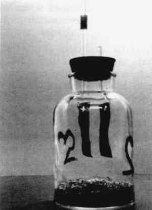
Besides the organic acid concentration in the test atmosphere, lead corrosion rate will depend on the temperature and humidity of the environment. For various reasons, the organic acid vapor concentration in the environment of wood and wood products will also be a function of temperature and humidity. It is desirable to keep the test period short so that organic acid concentration will not change due to secondary processes and so that results will be achieved quickly. The conditions used in this series of tests, 50�C and 80% RH, seemed the best compromise for accelerating the corrosion reaction without changing the mechanisms leading to the organic acid release or the lead corrosion. In atmospheres of 100% RH, small drops in temperature would cause condensation of water inside the wood, which can lead to biodeterioration (Schniewind 1989) and accompanying unpredictable changes in the acid release behavior. At temperatures in excess of 65�C, wood may become subject to thermal degradation processes (Wilcox 1989). For the conditions chosen, exposure times of two weeks were sufficient. More corrosive atmospheres and longer exposure times led to a loss of integrity of the test coupons.

3 EXPERIMENTAL PROCEDURES

CORROSION RATES were measured on clean, smooth coupons of chemically pure “assay” lead foil, cut to a standard size of 73 � 45 mm, with a hole of 8 mm diameter. The lead foil had a thickness of 0.1524 mm (0.006 in). Exposure of the coupons was done in 1000 ml glass bottles, suspended from glass hooks over 50 g (air dry) of the sample material or in empty bottles for the controls. One set of controls was used in every corrosion experiment. The exposure assembly, shown in figure 1, is virtually the same as that used by Clarke and Longhurst (1961) and others (Donovan and Stringer 1971; Donovan and Moynehan 1965). Their results showed that the use of rubber stoppers in the assembly does not accelerate corrosion. In all experiments reported here, except run 6, exposure conditions were 50�C and 80% RH. In experiment 6, temperature was 30�C and the humidity was cycled between 50% and 90% in 12-hour intervals.

Fig. 1. Exposure vessel used for corrosion experiments, with wood product samples and lead coupons in place

The lead coupons were degreased in acetone, pickled in boiling 1% acetic acid to remove all lead salts, rinsed under running water, and dried by dipping in acetone. The cleaning procedure closely follows ASTM standard G1-81 (1981). It was found in preliminary experiments that the suggested cleaning time of 5 minutes was excessive and that a 15-second wash was sufficient to remove all corrosion product, even from moderately corroded coupons. The cleaned coupons were weighed on an analytical balance (Sartorius Selectra) to the nearest 0.0001 g.

The wood product samples were cut into cubes of 1/2 in sides and subsequently comminuted in a Wiley mill to pass a 4 mesh screen. Milling was done to accelerate mixing of the vapors inside the wood with the surrounding air. Samples were weighed into the exposure bottles and kept in a controlled environment cabinet (AMINCO Climate-Lab Assembly) for 5 days before the start of the experiment. It had been shown previously that this time is sufficient for the samples to reach moisture equilibrium (Berndt 1987). At the end of the equilibration period, the bottles were closed with rubber stoppers holding the cleaned and weighed lead coupons and the exposure period started. At the end of the respective exposure times, bottles were withdrawn and the stoppers removed. The lead coupons were allowed to reach temperature equilibrium with the room air and then reweighed. The difference between weight before and after exposure was recorded as the weight gain.

In most experiments, the corroded lead coupons were cleaned again after weighing to determine the weight loss on exposure. As stated in ASTM standard G1-81 (1981), some metal is dissolved in this cleaning process and a correction has to be applied. The coupons were therefore subjected to the cleaning process seven times, and the mass loss plotted against the number of cleaning steps. A sample plot is shown in figure 2. If corrosion product removal is reasonably slow, the plot should show weight loss on washing at two different linear rates: first, a fast weight loss due to salt removal, giving a line through the origin: and second, a slower rate due to metal dissolution. The true weight of corrosion product removed would be the y-value of the intersection of the two lines.

Fig. 2. Example of a plot used for weight-loss determination

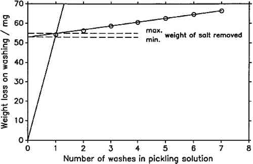
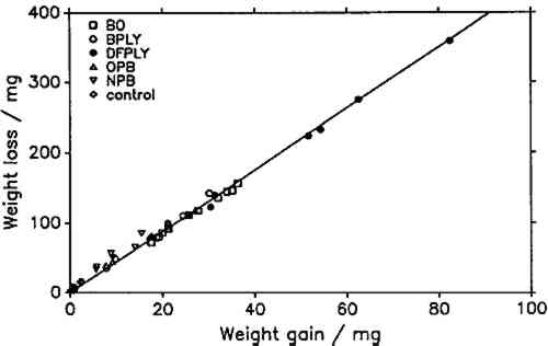
In this study, the line representing metal dissolution was determined by a linear regression on the last five data points of the cleaning series, since visual examination of the plots showed that these lay in all cases on a straight line. In figure 2, all seven points lie nearly on the regression line. This is representative for virtually all determinations carried out. Only when cleaning the most severely corroded coupons was there a significant deviation of the first one or two points from the fitted line. It was impossible in all cases to establish a rate of salt dissolution. As a compromise, a minimum and a maximum weight of the removed corrosion product were determined. The minimum was found from the y-intercept of the line fitted to the last five data points, assuming an infinitely fast rate of salt dissolution. The maximum was taken as the y-value of the intersection of the fitted line with the line through the origin and the first data point (fig. 2). Weight loss on exposure was calculated by subtracting the weight of salt removed from the weight after exposure and subtracting the result from the initial weight of the lead coupon.

As mentioned above, in all cases all points of the weight loss determination plots lay nearly on the metal-dissolution line. It can be assumed that the minimum weight loss is much closer to the true value than the maximum. Also, minimum and maximum weight loss rarely differed by more than the experimental error. Calculations and analyses were therefore based on minimum weight loss data.

The pH-values of the wood products, listed in table 1, were determined following the procedure outlined by Miles (1986). Twenty-five cc of the Wiley-milled samples and 150 cc of distilled water were agitated with a magnetic stirrer for 2 hours. After this time, the pH was measured with a Beckman pHI 45 pH meter by immersing a Beckman Futura II combination glass electrode and a thermocompensator in the stirred suspension and noting the stable instrument reading. Standard Beckman buffers of pH 4 (phthalate) and 7 (phosphate) were used for calibration. The reported values are averages of two independent measurements. Duplicate determinations did not vary by more than 0.05 pH units.

TABLE 1 Explanation of Sample Codes

4 STATISTICAL ANALYSIS

LINEAR REGRESSION analyses for best slope or best straight line were carried out conforming to standard practice (Bennet and Franklin 1954; Youden 1951). Regression coefficients and constants and their standard errors were calculated using built-in functions of Lotus 1-2-3, on an IBM PC AT. The 95% confidence intervals were calculated by multiplying the standard errors of the coefficients with the t-value for the appropriate number of degrees of freedom (Youden 1951, table 1).

5 RESULTS AND DISCUSSION

IF THE product of atmospheric lead corrosion is the same under all conditions, a plot of weight loss after exposure and cleaning against weight gain after exposure should yield a straight line through the origin. Figure 3 shows that this is indeed the case. Deviations from that line are of the order of magnitude of the experimental error. The slope of the line, the constant weight loss/weight gain ratio, is 4.387. Since the weight loss is equal to the mass of lead cations in the salt formed, and the weight gain is equal to the mass of salt anions, the weight gain/weight loss ratio is characteristic of the salt composition (Berndt 1987). The observed ratio is close to that expected for basic lead carbonate (2PbCO3Pb(OH)2, 4.02). It is significantly higher than for lead formate (Pb(HCOO)2, 2.3) or lead acetate (Pb(CH3COO)2, 1.75). This conforms with observations by Donovan and Moynehan (1965), who found that organic acid anions in salts formed over air drying paints made up about 0.02%–0.20% (by weight) of the salt. These organic acid anions were confined to the layer in intimate contact with the metal (Donovan and Stringer 1971).

Fig. 3. Weight loss of exposed and cleaned lead coupons vs. their weight gain after exposure. See table 1 for explanations of the sample codes.

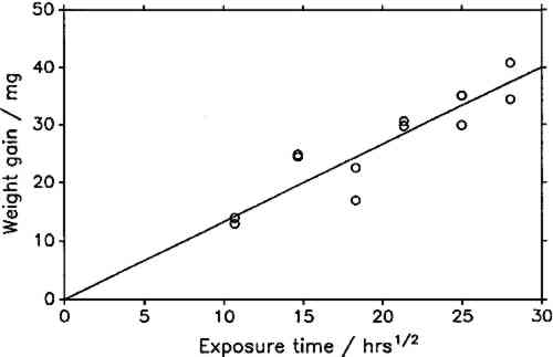
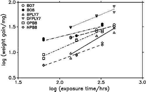
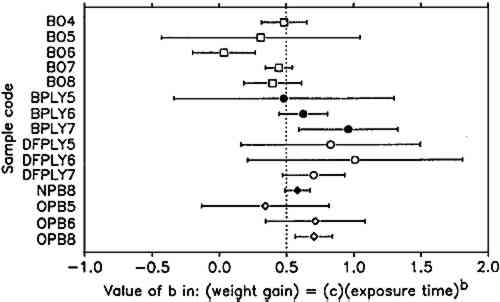
The constant weight loss/weight gain ratio also indicates that the corrosion mechanism was the same in all experiments. The corrosion rate is therefore a valid indicator of the organic acid concentration and atmospheric corrosiveness.

Since the weight gain is more than four times greater than the weight loss, it could be expected that weight gain determinations are more reliable because the weighing error is relatively smaller. That was found not to be the case. Errors from both types of determinations had the same relative magnitude, indicating that the observed errors are not due to lack of weighing precision but are caused by other variables, such as composition and temperature of the test atmosphere or state of the metal surface. Corrosion rates reported here were calculated from weight gain determinations.

Oak wood is known to corrode lead readily and was therefore chosen as the initial test material. It was found that the weight gain of lead on exposure to oak was proportional to the square root of exposure time (fig. 4). It was necessary to find out whether this is true for all other tested materials, that is, whether the value of b in equation 1 is 0.5 in all cases. Taking the logarithms of both sides of equation 1 yields:

Fig. .

Fig. 4. Weight gain of lead coupons exposed over California black oak vs. the square root of the expsure time

Fig. 5. Log-log plot of weight gain vs. exposure time, used to determine the exponent in the power law (weight gain) = (c) (exposure time)b. See table 1 for explanations of the sample codes.

Fig. 6. Comparison of values of the power law exponent b found for different wood products in different corrosion experiments. See table 1 for explanations of the sample codes.

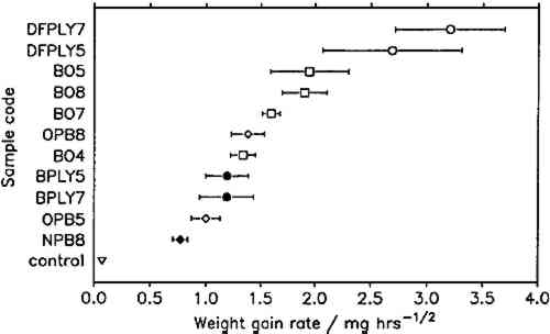
To compare corrosion rates caused by different wood products, the calculated weight gains were plotted against the square root of time and the best slope through the points was determined. The slopes (i.e., the corrosion rate constants) and their 95% confidence intervals for all comparable tests are presented in figure 7. Douglas fir plywood was clearly the most corrosive, and the recently purchased particleboard sample was the least corrosive of all tested wood products. Both results come as a surprise, given the bad reputations of particleboard and oak wood. A comparison of the pH values of the tested wood products (see table 1) with the corresponding corrosion rates confirms (cf. Donovan and Moynehan 1965) that pH is not an indicator of atmospheric corrosiveness.

Fig. 7. Comparison of weight gain rates caused by various wood products in different corrosion experiments, with the assumption of a constant power law exponent, b = 0.5. See table 1 for explanations of the sample codes.

No attempts were made to characterize the samples further than by type of product, pH, and wood species, as given in table 1, since this series of experiments was planned as a trial for the feasibility and sensitivity of this atmospheric corrosion test. The results reported here cannot be generalized with regard to wood species, product, length of storage, or other independent factors.

It appears that corrosive emissions increase with the time between sample preparation (cutting and milling) and the corrosion tests. Birch plywood gave the same corrosion rate in two successive tests, but the other duplicates from identical batches (BO4/BO5, BO7/BO8, DFPLY5/DFPLY7, OPB5/OPB8), all have a higher corrosion rate in the later test. This phenomenon should be investigated systematically in future experiments.

Figure 5 shows that the experimental error of the corrosion rate determination is roughly proportional to the rate itself and usually of acceptable magnitude. In all experiments so far, the test had to be terminated for a given exposure bottle to measure weight changes. This significantly limited the number of experimental points available for corrosion rate determinations, from as low as two test coupons each at two exposure times (all materials in run 5) to at most two test coupons each after six exposure times. As mentioned above, the corrosion rate can be confidently determined and compared for various materials on the basis of weight gain measurements alone. It is therefore possible to make use of continuous weight gain measurement, for example, by suspending the test coupons from an automatic balance. This would increase the number of experimental points available for the rate determination significantly and could be expected to narrow the confidence interval for the calculated rate.

It was originally planned to correlate the corrosion rate in the presence of wood products to that in the laboratory atmosphere at the same temperature and humidity to correct for differences in the “background” corrosiveness (Berndt 1987). This plan proved to be impractical, since the error in the background corrosion rate determinations was greater than any differences found in four experiments. Weight changes were clearly measurable, however, even in the controls.

6 SUMMARY AND CONCLUSIONS

THE TENDENCY of microclimates in the vicinity of wood and wood products to corrode lead can be measured by following the weight gain of standard test coupons with exposure time at a temperature of 50�C and a RH of 80%. It can reasonably be assumed that for all tested materials the amount of metal oxidized per unit surface area is directly proportional to the square root of the exposure time.

Corrosiveness of atmospheres in the vicinity of wood products varies significantly with the type of wood product but is not correlated with the pH of the wood product. In the worst case, corrosion was accelerated by a factor of 46, compared to the average corrosiveness of the laboratory air under test conditions. The least offensive material accelerated corrosion by a factor of 11. Corrosiveness seems to increase slightly with the time between sample preparation (milling) and the corrosion test. Treatment and storage effects on corrosiveness need further systematic investigation.

The results of this study cannot be generalized with regard to wood species, product, length of storage, or other independent factors. Testing of individual batches of materials is preferable to any “rule of thumb.” The procedure used in this study seems reliable, simple, and fast enough to allow routine tests of potential construction materials.

Corrosion rate measurement by the method described here is less intrusive than an estimation of corrosiveness by measuring atmospheric composition, since no appreciable amounts of trace gases or vapors are adsorbed or consumed due to reaction. According to previous reports (Clarke and Longhurst 1961), lead corrosion is significantly accelerated by acetic acid concentrations as low as 0.5 ppm. To detect such low concentrations using gas analysis, sample volumes of 20 liters and more are usually required (Devorkin et al. 1972; Budde and Eichelberger 1979). Corrosion rate measurement with lead coupons can be carried out in air spaces with a volume of less than 1 liter.

All organic materials can be expected to decompose at some rate, while releasing organic acids. This has been shown not only for wood products but also for various types of coatings (Donovan and Moynehan 1965). The atmospheric corrosion test proposed here is a reasonably fast and reliable way of testing storage and display systems. The tests would be particularly convenient if weight gain measurements were carried out continuously, using an automatic balance in the test environment.

REFERENCES

ASTM. 1981. Preparing, cleaning, and evaluating corrosion test specimens, G1-81; Conducting atmospheric corrosion tests on metals, G50-76. In Annual book of ASTM standards: Wear and erosion, vol. 03.02, Metal corrosion. Philadelphia: American Society for Testing and Materials.

Arni, P. G., G. C.Cochrane, and J. D.Gray. 1965a. The emission of corrosive vapours by wood, I: Survey of the acid-release properties of certain freshly felled hardwoods and softwoods. Journal of Applied Chemistry15: 305–13.

Arni, P. G., G. C.Cochrane, and J. D.Gray. 1965b. The emission of corrosive vapours by wood, II. The analysis of the vapours emitted by certain freshly felled hardwoods and softwoods by gas chromatography and spectrophotometry. Journal of Applied Chemistry15: 463–68.

Bennet, C. A., and N. L.Franklin. 1954. Statistical analysis in chemistry and the chemical industry. New York: John Wiley and Sons.

Berndt, H.1987. Assessing the detrimental effects of wood and wood products on the environment inside display cases. AIC preprints, 15th Annual Meeting, American Institute for Conservation, Vancouver, British Columbia. 22–33.

Blackshaw, S. M.1982. The testing of display material. Museum Ethnographers Group occasional paper no. 1. 40–45.

Blackshaw, S. M., and V. D.Daniels. 1978. Selecting safe materials for use in the display and storage of antiquities. ICOM Committee for Conservation preprints, 5th Triennial Meeting, Zagreb, 23/2/1–23/2/9.

Budde, W. L., and J. W.Eichelberger. 1979. Organics analysis using gas chromatography/mass spectrometry: A techniques and procedures manual. Ann Arbor, Mich: Ann Arbor Science Publishers.

Carpenter, J. M., and P. B.Hatchfield. 1987. Formaldehyde: How great is the danger to museum collections?Cambridge, Mass.: Center for Conservation and Technical Studies, Harvard University Art Museums.

Clarke, S. G., and E. E.Longhurst. 1961. The corrosion of metals by acid vapours from wood. Journal of Applied Chemistry11: 435–43.

Connolly, M. D.1987. Creating microenvironments in airtight cabinets—a warning: Statement of preliminary findings. AIC Newsletter12(4):5–6.

Devorkin, H., R. L.Chass, and A. P.Fudurich. 1972. Air pollution source testing manual. Los Angeles County, Calif: Air Pollution Control District.

Donovan, P. D., and J.Stringer. 1969. Corrosion of metals by acid vapors. Extended abstracts, 4th International Congress on Metallic Corrosion, Amsterdam, The Netherlands. 133–36.

Donovan, P. D., and J.Stringer. 1971. Corrosion of metals and their protection in atmospheres containing organic acid vapours. British Corrosion Journal6: 132–38.

Donovan, P. D., and T. M.Moynehan. 1965. The corrosion of metals by vapours from air-drying paints. Corrosion Science5: 803–14.

FitzHugh, E. W., and R. J.Gettens. 1971. Calclacite and other efflorescent salts on objects stored in wooden museum cases. In Science and archaeology, ed.R. H.Brill. Cambridge, Mass: MIT Press. 91–102.

GCI. Newsletter.1987. Microenvironmental research. Getty Conservation Institute Newsletter2(3):7.

GCI. Newsletter. 1988. Environmental research in conservation. Getty Conservation Institute Newsletter3(2): 1–2.

Hatchfield, P. B., and J. M.Carpenter. 1986. The problem of formaldehyde in museum collections. International Journal of Museum Management and Curatorship5: 183–88.

Leveque, M. A.1986. The problem of formaldehyde: A case study. AIC preprints, 14th Annual Meeting, American Institute for Conservation, Washington, D.C.56–65.

Miles, C. E.1986. Wood coatings for display and storage cases. Studies in Conservation31: 114–24.

Oddy, W. A.1973. An unsuspected danger in display. Museums Journal73: 27–28.

Oddy, W. A.1975. The corrosion of metals on display. In Conservation in archaeology and the arts, ed.N. S.Brommelle and P.Smith. London: International Institute for Conservation of Historic and Artistic Works. 235–37.

Packman, D. F.1957. Corrosion of cadmium plated steel by plywood and wood assemblies made with synthetic resin glues. Forest Products Research Laboratory report 77646.

Packman, D. F.1960. The acidity of wood. Holzforschung14: 178–83.

Padfield, T., D.Erhard, and W.Hopwood. 1982. Trouble in store. In Science and technology in the service of conservation, ed.N. S.Brommelle and G.Thomson. London: International Institute for Conservation of Historic and Artistic Works. 24–27.

Schniewind, A. P.1989. Strength. In Concise encyclopedia of wood and wood-based materials, ed.A. P.Schniewind. Cambridge, Mass: MIT Press. 245–50.

Scully, J. C.1975. The fundamentals of corrosion. Oxford: Pergamon Press.

Thomson, G.1978. The museum environment. London: Butterworths.

Weast, R. C., ed.1979. CRC handbook of chemistry and physics, sec. B. Boca Raton, Fla.: CRC Press.

Wilcox, W. W.1989. Decay during use. In Concise encyclopedia of wood and wood-based materials, ed.A. P.Schniewind. Cambridge, Mass: MIT Press. 71–75.

Youden, W. J.1951. Statistical methods for chemists. New York: John Wiley and Sons.

AUTHOR INFORMATION

HARALD BERNDT has been assistant specialist at the University of California Forest Products Laboratory, Wood Artifacts Conservation and Timber Mechanics Group, since 1985. He is the 1989–90 vice president/program chair of the Bay Area Art Conservation Guild. He holds an M.S. degree in wood science and technology from the University of California, Berkeley, and the degree of Diplom-Holzwirt from the University of Hamburg, Germany. He has published articles in the ACS Symposium Series, Journal of Wood Conservation, and AIC preprints. Address: University of California at Berkeley, Forest Products Laboratory, 1301 South 46th St., Richmond, Calif. 94804.

Section Index