The Arrhenius Equation
Foundation for Advancement in Conservation
© 2008
Introduction
In 1889 the Swedish scientist Svante Arrhenius put forward the concept of activation energy. The Arrhenius equation links activation energy to the rate of the reaction. Conservators and conservation scientists use the Arrhenius equation to predict how materials will behave over time.
Before starting this unit make sure you feel comfortable with:
- Graphs
- Straight line graphs
- Labeling axes
- Basic algebra
- Simple equations
- Exponentials
Contents
This tutorial is divided into the following sections:
Please complete each section in order, as the information builds on that covered in previous sections. You can return to any section later.
Press Ctrl+Shift+F to search.
Learning Objectives
After completing this tutorial, you will be able to:
- List the three main methods of accelerating aging in conservation research
- Define rate of reaction
- Describe a method of determining the rate of reaction
- Define the components of the Arrhenius equation
- Understand how a straight-line equation derived from the Arrhenius equation is used to calculate reaction rates
- Cite the limitations of the Arrhenius equation
Svante August Arrhenius (1859–1927)

He was something of a mathematics prodigy and studied at the Swedish Academy of Science in Stockholm. However, when he submitted his doctoral thesis on electrolytic conductivity, it was given the lowest mark possible for him to be able to pass.
This work later earned him the Nobel prize in chemistry.
Work of Arrhenius
In 1889 Arrhenius put forward the concept of activation energy. The Arrhenius equation links activation energy to the rate of the reaction.
In 1904 he gave a series of lectures at the University of California on the theory of toxins and antitoxins that was later published with the title "Immunochemistry".
Among his many other interests Arrhenius developed a theory to explain ice ages. He thought changes in the levels of carbon dioxide in the atmosphere would alter the surface temperature of the Earth through a greenhouse effect.
Types of Simulated Aging
Conservators and conservation scientists use the Arrhenius equation to predict how materials will behave over time.
There are three main methods of accelerated aging that are used in conservation research:
- Thermal aging: where samples are kept in a thermally controlled oven at either a stable or ramped relative humidity.
- Light aging: where samples are exposed to high intensity light and/or UV light.
- "Pollution" aging: where the samples are kept in a sealed chamber and subject to nitrogen or sulfur pollution.
The Arrhenius equation is generally used with thermal aging.
Rates of Reactions
To begin, we will look at rates of reactions.
Chemists are not only interested in the results of chemical reactions, but also in measuring how fast the reaction will go.
To calculate the rate of reaction remember:

\(\frac{\text{Rise}}{\text{Run}}\)
\(\text{The rate of a reaction } = \frac{\text{The difference in y}}{\text{The difference in x}}\)
\(x\) and \(y\) represent whatever qualities you are measuring:
- Yellowing vs. time
- Immiscibility vs. concentration
- Work done vs. # conservators
Which reaction is faster?
 Note: The scale is the same for both graphs.
Which reaction is faster?
Note: The scale is the same for both graphs.
The graph on the right represents the faster reaction rate. It has a larger slope (rise/run) than the graph on the left.
How to Measure a Rate of Reaction
Let's briefly look at how the rate can be measured. If we take a simple reaction:

We can now use a concentration of alcohol that is far in excess of the acid, then we can stop the reaction at set times and measure the concentration of the acid (reactant) or the concentration of the ester (product).
Measuring a Reaction Rate

In this reaction one molecule of acid reacts with one molecule of alcohol to produce one molecule of ester (and one molecule of water).
Since the acid and alcohol are in a liquid (aqueous) state, the final concentration of the water can be ignored.
If, instead of mixing equal amounts of acid and alcohol, we add a huge excess of alcohol, then we can assume that the concentration of the alcohol doesn't really change as the reaction progresses. This makes it easier to follow the change in the acid.
Changes in Concentration of Reactants and Products
As the concentration of the acid decreases, the concentration of the ester increases.

\(\text{Rate of reaction } = -\frac{\text{[acid]}}{time} \quad \text{Rate of reaction } = \frac{\text{[ester]}}{\text{time}}\)
Square brackets usually mean "concentration of"
The Rate Constant k
Every chemical reaction has a rate constant \(k\).
This is calculated from the kind of experiment we looked at that followed the concentrations of the acid and ester as the reaction progressed.
acid + alcohol  ester + water
All reactions are, in theory, capable of going both ways. In this case we are assuming that everything ends up on the right of the arrows
Rate of reaction = \(k\) [acid]
If all the acid and alcohol react and produce the ester then we can calculate the rate at which that happens from the concentration of the acid.
Simplified Treatment
If you have studied this previously, you know that I have carefully oversimplified what is a fairly complex set of mathematical concepts.
As used by conservators, the Arrhenius equation takes the form of a pseudo-first order rate equation, and that is where this tutorial is leading.
I am also deliberately avoiding the use of calculus. The derivation of the rate equations can be found in any book on physical chemistry or on Wikipedia.
Relating Rate Constant to Temperature
The Arrhenius equation is very useful as a means by which we can relate the rate constant for a reaction to the temperature at which the reaction is taking place.
\(k = Ae^{-\frac{Ea}{RT}} \)
\(k\) is the rate constant for the reaction.
\(T\) is the temperature at which the reaction is taking place.
Explanation of the Equation
\(k = Ae^{-\frac{Ea}{RT}} \)
\(k\) is the rate constant for the reaction. This is the value that we would like to measure in order to predict some aging characteristic of an artwork.
\(A\) is the pre-exponential constant for the reaction. This is a constant that we will calculate experimentally as described later in the tutorial.
Explanation of the Equation
\(k = Ae^{-\frac{Ea}{RT}} \)
\(e\) is the exponential function of the natural log \(\ln\).
\(Ea\) is the activation energy for the reaction. All chemical reactions have an energy barrier that must be overcome before the reaction can proceed.
Explanation of the Equation
\(k = Ae^{-\frac{Ea}{RT}} \)
\(R\) is used to represent either the Boltzmann constant or the gas constant, depending on the units of measure used for the activation energy.
\(T\) is the temperature measured in Kelvin.
Explanation of the Equation: Pre-Exponential Factor & Activation Energy
 Pre-exponential Factor: This is a constant and is different for each individual reaction. It is calculated from the graph that will come later in this tutorial.
Activation Energy: All chemical reactions have an energy barrier before the reaction can proceed. This is the activation energy.
Explanation of the Equation: Temperature
The temperature is measured in Kelvin. To convert Celsius into Kelvin:
\(K = x ºC + 273.15\)
To convert Fahrenheit to Kelvin:
\(K = \frac{5(x ºF + 459.67)}{9}\)
Explanation of the Equation: Boltzmann Constant
Boltzmann constant = 1.3806504x10⁻²³ joules/Kelvin
The Boltzmann constant is used if the activation energy for the reaction is given in joules per molecule.
If the activation energy is in joules per mole then the gas constant is used.
Gas constant = 8.314472 joules/Kelvin per mol
Explanation of the Equation: The Exponential Function
\(e\) is the exponential function of the natural log \(\ln\).
In the Arrhenius equation \(A\) is called the pre-exponential factor—the factor before the exponential \(e\).
Logs allow a simplified way of manipulating numbers.
\(y = 2\)
\(b=10\)
\(x=100\)
\(y = \log_{b} x\)
\(x = b^y\)
\(2 = \log_{10} 100\)
\(100 = 10^2\)← exponential
The natural log, which is the progression most often found in nature, is \(\log_{2.718}\). Scientific calculators will calculate logs and natural logs.
Manipulating the Equation to Straight Line Formula
We can manipulate the Arrhenius equation by taking the natural log of both sides. The result is:
\(\ln k = \ln A + \frac{-E_a}{R} \times \frac{1}{T}\)
And this is in the form of an equation for a straight line graph:
\(y = mx + c\)
\(\ln k = \frac{-E_a}{R}\ \frac{1}{T} + \ln A\)
General Equation for a Straight Line
If any of your data can be manipulated into the form:
\(y = mx + c \)
then a graph of that data will be a straight line with \(m\) as the slope of the line and \(c\) as the intercept on the \(y\) axis.

If your data fitted the equation \(y = 2x + 1\) the graph would be:
Quick Math Review
Try out this quick math review.

\[y = \_\_x + \_\_\]
\[y = -2 x + 4\]
The slope is \(\frac{\text{difference in }y}{\text{difference in }x}\)
In this case the difference in \(y\) is \(1-4=-4\). The difference in \(x\) is \(2-0=2\).
So the slope is \(-\frac{3}{2}=-1.5\)
The intercept is \(4\).
Using the Straight-Line Graph to Find the Activation Energy
Plotting \(\ln k\) versus \(\frac{1}{T}\) will give a straight line graph with a slope \(-E_a/R\) and the \(y\)-intercept \(\ln A\).

Extrapolation: \(\ln A\) can be read on the \(y\) axis where the lines meet.
The slope of this line (\(\frac{\text{Rise}}{\text{Run}}\)) gives \(\frac{-E_a}{R}\)
By extrapolating the line back to the \(y\) axis we can find \(\ln A\) for the reaction and the slope divided by \(R\) will give the activation energy.
Conservators generally use the Arrhenius equation with accelerated thermal aging.
Sample Experiment
Let's imagine we were going to use the Arrhenius equation to compare the stability of three different kinds of paper A, B, C.
First we have to choose a method of determining how the papers have changed—in this case fold endurance (how many times a paper can be folded before it breaks).
Sample Experiment
Then we have to run at least 3, and preferably more, accelerated aging tests for each paper, taking some samples out regularly and testing them.
| Run | ºC | Paper A | Paper B | Paper C |
|---|---|---|---|---|
| 1 | 60 | A1 | B1 | C1 |
| 2 | 70 | A2 | B2 | C2 |
| 3 | 80 | A3 | B3 | C3 |
| 4 | 90 | A4 | B4 | C4 |
There are 12 sets of samples to be tested and we will take out a percentage of each set on days 10, 20, 40, 60, and 100 to test for fold endurance.
Sample Experiment
Plot the fold endurance against time for each sample in each run.
Find \(k\), the rate of reaction from the slope of each line.

Sample Experiment

You may get an S shaped curve rather than a nice straight line.
This is the point of inflection where the slope of the line changes from convex to concave.
Sample Experiment
You will end up with a table of \(k\) values calculated from the slopes of each sample.
Use these values to plot changes in the rate of reaction with the temperature and compare the papers.
| Run | ºC | Paper A | Paper B | Paper C |
|---|---|---|---|---|
| 1 | 60 | \(k_{A1}\) | \(k_{B1}\) | \(k_{C1}\) |
| 2 | 70 | \(k_{A2}\) | \(k_{B2}\) | \(k_{C2}\) |
| 3 | 80 | \(k_{A3}\) | \(k_{B3}\) | \(k_{C3}\) |
| 4 | 90 | \(k_{A4}\) | \(k_{B4}\) | \(k_{C4}\) |
Sample Experiment
Plot \(\ln k\) against temperature for each paper.
You can extrapolate to room temperature and determine the relative stabilities of the papers.

Example from the Literature
 Let's look at an actual example of using the Arrhenius equation from the literature.
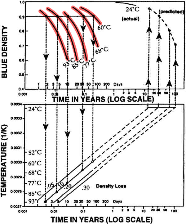
Here are the results of thermally aging photographs to predict density loss over time by Anderson and Ellison (1992).
There are two graphs. First the authors ran a series of 5 tests at different temperatures (93, 85, 77, 68, 60 ºC) to find the rate of density loss in photographs.
Example from the Literature
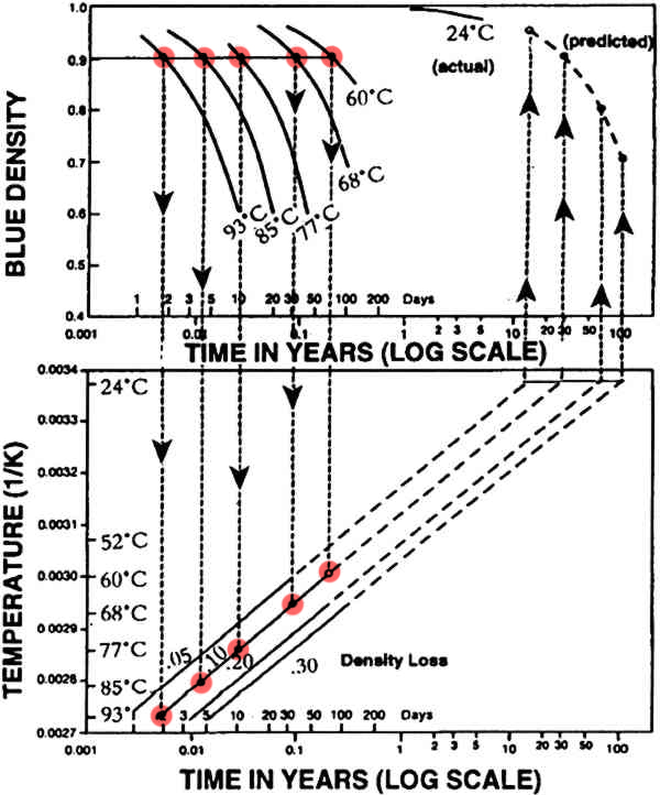
Next they chose points at which the density loss for each sample was the same, 0.005%, 0.1%, 0.2%, 0.3%. (The 0.1% loss is highlighted in the diagram.)
They plotted these points on the second graph of temperature versus time. Note the temperature decreases up the y axis.
Example from the Literature
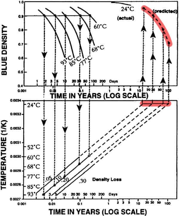
Finally they extrapolated the lines showing loss of density to 24 ºC (room temperature) highlighted on the straight line, and plotted these points on the first graph to predict the loss of density in photographs at room temperature, highlighted on the curved lines.
Limitations
There are some well-known limitations to the Arrhenius equation:
- The rate of reaction has to be constant over the time involved.
- Different modes of failure may happen at different times and this will affect the rate of reaction.
- All of the changes over time may not take place at the same rate.
- There may be competing reactions taking place.
- The activation energy has to be independent of temperature.
- There is a discontinuity in an Arrhenius plot around the glass transition temperature (\(T_g\)).
Arrhenius Equation: Summary
In this tutorial you have learned about:
- The three main methods of accelerated aging in conservation research
- How to define rate of reaction
- A method of determining the rate of reaction
- The definition of the components of the Arrhenius equation
- How a straight-line equation derived from the Arrhenius equation is used to calculate reaction rates
- The limitations of the Arrhenius equation
References
This article, which uses the Arrhenius equation to examine changes in photographs, can be found at JAIC Online
Credits
Researched and written by Sheila Fairbrass Siegler
Instructional Design by Cyrelle Gerson of Webucate Us
Project Management by Eric Pourchot
Special thanks to members of the Association of North American Graduate Programs in Conservation (ANAGPIC) and the AIC Board of Directors for reviewing these materials.
This project was conceived at a Directors Retreat organized by the Getty Conservation Institute and was developed with grant funding from the Getty Foundation.
Converted to HTML5 by Avery Bazemore, 2021
© 2008 Foundation for Advancement in Conservation